Research
Pushing the frontiers of AI for equitable innovation through autonomous research groups.

Research Areas
Knowledge Representation & Reasoning
Computer Vision
Natural Language Processing
Federated & Privacy- Preserving Learning
Multimodal AI
Speech & Audio Processing
Learning Algorithms & Optimization
Expand human knowledge through high-integrity research that pushes the frontiers of AI.
Address critical real-world challenges where AI can create valuable impact.
Ensure benefits of AI reach everyone and its progress is shaped by all.


Our Impact
0+
publications in top-tier venues
$0.0M+
research funding accross 9 international grants
0%
international collaboration rate
0
open-source repositories impacting the AI community
Featured Projects
AI-Powered Task-Shifting for High-Quality Fetal Ultrasound Service in Community Healthcare Settings
AI-Powered Task-Shifting for High-Quality Fetal Ultrasound Service in Community Healthcare Settings
Computer Vision | Healthcare Task-Shifting | Low-Resource AI | AI in Maternal & Reproductive HealthRKDB
AI-Enhanced Coronary Artery Disease Diagnostics from X-Ray Angiography
AI-Enhanced Coronary Artery Disease Diagnostics from X-Ray Angiography
Medical Image Analysis | Computer Vision | Clinical Decision Support | Low-Resource AIYRDBSB
+1
Systems Genomics Modeling of Multi-drug Resistance in Mycobacterium tuberculosis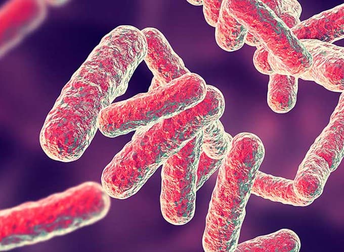
Systems Genomics Modeling of Multi-drug Resistance in Mycobacterium tuberculosis
Computational Genomics | Infectious Disease Genomics | Drug Resistance ModelingLead:
DSDRDB
+1

AI-Powered Surgical Planning for Knee Osteotomy
AI-Powered Surgical Planning for Knee Osteotomy
Medical Image Analysis | Computer Vision | Clinical Decision Support | Precision MedicineAI-Assisted Diarrheal Parasite Detection with Smartphone Microscopy
AI-Assisted Diarrheal Parasite Detection with Smartphone Microscopy
Medical Image Analysis | Computer Vision | Infectious Disease Genomics | Low-Resource AI | Public HealthUCST
Feature Publications
2023
FUTURE-AI: International consensus guideline for trustworthy and deployable artificial intelligence in healthcare
Karim Lekadir, Bishesh Khanal, Martijn Starmans
arXiv preprint arXiv:2309.12325 , 2023
2025
Transforming healthcare through just, equitable and quality driven artificial intelligence solutions in South Asia
Sushmita Adhikari, Iftikhar Ahmed, Deepak Bajracharya, Bishesh Khanal, Chandrasegarar Solomon, Kapila Jayaratne, Khondaker Abdullah Al Mamum, Muhammad Shamim Hayder Talukder, Sunila Shakya, Suresh Manandhar, Zahid Ali Memon, Moinul Haque Chowdhury, Ihtesham ul Islam, Noor Sabah Rakhshani & M. Imran Khan
npj Digital Medicine (nature)
Peer Reviewed Journal articleTOGAI (Transforming Global Health with AI)
2025
Assistive Artificial Intelligence in Epilepsy and Its Impact on Epilepsy Care in Low- and Middle-Income Countries
Nabin Koirala, Shishir Raj Adhikari, Mukesh Adhikari, Taruna Yadav, Abdul Rauf Anwar, Dumitru Ciolac, Bibhusan Shrestha, Ishan Adhikari, Bishesh Khanal, Muthuraman Muthuraman
Brain Sciences (MDPI) 2025
Peer Reviewed Journal articleTOGAI (Transforming Global Health with AI)
2025
Multimodal Federated Learning With Missing Modalities through Feature Imputation Network
Pranav Poudel, Aavash Chhetri, Prashnna Gyawali, Georgios Leontidis, Binod Bhattarai
Medical Image Understanding and Analysis (MIUA) 2025
Peer Reviewed Conference articleBBMMLL (B Bhattarai Multi-Modal Learning Lab)
2024
NLPineers@ NLU of Devanagari Script Languages 2025: Hate speech detection using ensembling of BERT-based models
Anmol Guragain, Nadika Poudel, Rajesh Piryani, Bishesh Khanal
CHiPSAL: Challenges in Processing South Asian Languages. COLING 2025
Peer Reviewed Workshop articleTOGAI (Transforming Global Health with AI)


.jpg&w=1080&q=75)

